Correcting plate position for hit-calling and profiling

Position effects are real. Edge wells evaporate, corners sit at a different temperature, and dispensing drifts along a row. mt.pp.correct_plate_position removes a plate’s row and column effects with a two-way median polish (Tukey), which a few extreme wells cannot distort. Whether you should correct depends on what you measure. A single readout is one number per well, as in a biochemical hit screen. A multivariate profile is hundreds of morphology features per well.

The default method, b_score (Brideau et al. [2003]), divides the median-polish residual by the plate’s median absolute deviation (MAD), which gives a robust position-corrected z-score per plate. The median_polish method subtracts the effects and keeps the data’s units. On a single readout the correction recovers hits that a gradient hides. On a multivariate profile it lowers compound retrieval. The correction helps for hit-calling against a gradient, and it does not help for multivariate profiling.

import warnings

import anndata as ad
import matplotlib.pyplot as plt
import numpy as np
import pandas as pd

import mantispy as mt
from mantispy._core.plate import PLATE_FORMATS, well_col, well_name, well_row
from mantispy._core.schema import stamp

warnings.filterwarnings("ignore")

Hit-calling on a single readout

On a single readout a gradient can hide real hits. An active well in a cool corner reads lower than an inactive well in a warm corner. The plate below is synthetic. It has a strong row and column gradient, six real hits placed at random, and otherwise-inactive wells. We score the result by how many of the six hits land in the top six wells, which we call precision at six.

n_rows, n_cols = PLATE_FORMATS[96]
names = [well_name(r, c) for r in range(n_rows) for c in range(n_cols)]
rows = np.array([well_row(w) for w in names], dtype=float)
cols = np.array([well_col(w) for w in names], dtype=float)
rng = np.random.default_rng(0)

gradient = 6.0 * rows / rows.max() + 4.0 * cols / cols.max()
readout = gradient + rng.normal(0.0, 0.3, len(names))
hits = rng.choice(len(names), size=6, replace=False)  # six real hits, scattered at random
readout[hits] += 3.0  # a randomized layout, as B-score assumes

plate = ad.AnnData(
    X=readout.reshape(-1, 1).astype(np.float32),
    obs=pd.DataFrame(
        {"Metadata_Plate": "demo", "Metadata_Well": names, "Metadata_Control": True},
        index=[str(i) for i in range(len(names))],
    ),
    var=pd.DataFrame(index=["readout"]),
)
stamp(plate, resolution="well")
scored = mt.pp.correct_plate_position(plate, method="b_score", copy=True)


def hit_precision(values, k=6):
    """Share of the true hits among the top-k wells -- how we measure whether correction helped."""
    return len(set(np.argsort(values)[::-1][:k]) & set(hits.tolist())) / k


raw_precision = hit_precision(readout)
b_precision = hit_precision(np.asarray(scored.X, dtype=float)[:, 0])

fig, axes = plt.subplots(1, 2, figsize=(10, 3.6), layout="constrained")
mt.pl.plate(plate, color="readout", plate="demo", ax=axes[0])
axes[0].set_title(f"raw  (hit precision@6 = {raw_precision:.2f})", fontsize=10)
mt.pl.plate(scored, color="readout", plate="demo", ax=axes[1])
axes[1].set_title(f"B-score  (hit precision@6 = {b_precision:.2f})", fontsize=10)
plt.show()

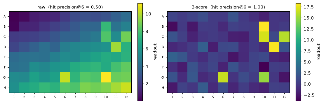
Raw, the gradient lifts warm-corner background above hits in cool wells, so some hits miss the top six. After the B-score the gradient is gone and the six hits are the top six, with the precision shown in the panel titles. The B-score works here because four conditions hold. First, the data is a single readout. Second, the task is hit-calling. Third, the layout is randomized. Fourth, most wells are inactive. On a profile the conditions do not hold, which the rest of the page shows.

Multivariate profiling

A morphological profile is different. It is hundreds of correlated features per well, where position is a small part and the biology is each compound’s full multivariate shift. The shift has to stay comparable across plates and laboratories. The plates below are five from one laboratory (source_4) that carry a real position artifact and five from other laboratories that do not. Each plate is normalized against its DMSO negative controls (negcon) with mad_robustize, which centres on the median and scales by the MAD. detect_plate_position scores each plate by cross-validation. It fits the row and column effects on part of the control wells and checks how well they predict the held-out controls, reported as cv_r2_median. The column frac_features_positive is the share of features where that prediction beats the plate mean. A score above zero means the pattern generalizes.

flagged = ["BR00126113", "BR00126114", "BR00126115", "BR00126116", "BR00126117"]
clean = ["JCPQC051", "ACPJUM012", "1053600674", "GR00003394", "CP1-SC1-25"]
jump = mt.ds.jump_target2(plates=flagged + clean)
mt.pp.normalize(jump, method="mad_robustize", by="Metadata_Plate", reference="negcon")
mt.pp.feature_select(jump, na_cutoff=0.0)
jump = mt.pp.subset_features(jump)

mt.pp.detect_plate_position(jump, reference="negcon")
detection = jump.uns["mantispy"]["plate_position_detection"].copy()
source = jump.obs.drop_duplicates("Metadata_Plate").set_index(
    jump.obs.drop_duplicates("Metadata_Plate")["Metadata_Plate"].astype(str)
)["Metadata_Source"]
detection["source"] = detection["plate"].map(source.to_dict())
detection.sort_values("cv_r2_median", ascending=False).round({"cv_r2_median": 3, "frac_features_positive": 3})

	plate	n_controls	cv_r2_median	frac_features_positive	reason	source
2	BR00126113	64	0.784	0.823		source_4
5	BR00126116	64	0.754	0.789		source_4
4	BR00126115	64	0.712	0.795		source_4
6	BR00126117	64	0.710	0.793		source_4
3	BR00126114	64	0.504	0.651		source_4
8	GR00003394	256	-0.129	0.307		source_9
7	CP1-SC1-25	64	-0.545	0.153		source_7
9	JCPQC051	64	-0.659	0.169		source_3
1	ACPJUM012	64	-0.825	0.026		source_5
0	1053600674	65	-0.839	0.084		source_2

scored = detection.dropna(subset=["cv_r2_median"]).sort_values("cv_r2_median")
palette = dict(zip(sorted(scored["source"].unique()), plt.cm.tab10.colors, strict=False))

fig, ax = plt.subplots(figsize=(6, 4), layout="constrained")
ax.barh(range(len(scored)), scored["cv_r2_median"], color=[palette[s] for s in scored["source"]])
ax.axvline(0.0, color="black", lw=1)
ax.set_yticks(range(len(scored)), scored["plate"], fontsize=7)
ax.set_xlabel("cross-validated R² of the row/column fit (cv_r2_median)")
ax.legend(
    handles=[plt.Line2D([], [], marker="s", ls="", color=c, label=s) for s, c in palette.items()],
    fontsize=7,
    loc="lower right",
    title="source",
)
plt.show()

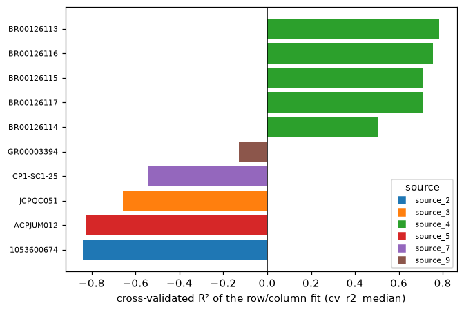
The five source_4 plates score well above zero and the others score below it. The artifact is real and specific to one laboratory. A positive score means the row and column pattern is stable across control wells. It does not mean correcting the plate will help the biology, which the retrieval test below settles. A high score is also a quality-control signal, so on a profiling screen, excluding or inspecting the plate is usually better than correcting it. In a scan of the full 141-plate Target-2 set only six plates scored positive, and five of them came from this one laboratory, so correcting every plate would change them all to address a few.

The scores summarize the plates, and the figure below shows the structure itself. We average the most position-correlated features into one signal and show the control wells only, because on treated wells the compound moves the signal and hides the field. The flagged plate has coherent spatial structure, a clean plate from another laboratory has scattered noise, and median polish flattens it.

flagged_plate, clean_plate = "BR00126113", "JCPQC051"
controls = jump[(jump.obs["Metadata_Plate"].astype(str) == flagged_plate) & jump.obs["Metadata_Control"].to_numpy()]
cv = np.asarray(controls.X, dtype=float)
crows = np.array([well_row(w) for w in controls.obs["Metadata_Well"]], dtype=float)
ccols = np.array([well_col(w) for w in controls.obs["Metadata_Well"]], dtype=float)


def position_score(column):
    """Combined absolute correlation of a feature's control values with well row and column."""
    row_r = np.corrcoef(crows, column)[0, 1] if np.ptp(column) > 0 else 0.0
    col_r = np.corrcoef(ccols, column)[0, 1] if np.ptp(column) > 0 else 0.0
    return abs(np.nan_to_num(row_r)) + abs(np.nan_to_num(col_r))


# average the 40 most position-correlated features into one signal, so single-feature outliers do not dominate
top = np.argsort([position_score(cv[:, j]) for j in range(cv.shape[1])])[::-1][:40]


def signal(adata):
    """Mean of the most position-correlated features, as one position signal per well."""
    return np.asarray(adata.X, dtype=np.float64)[:, top].mean(axis=1)


jump.obs["position signal"] = signal(jump)
corrected = mt.pp.correct_plate_position(
    jump, method="median_polish", reference="negcon", plates=[flagged_plate], copy=True
)
corrected.obs["position signal"] = signal(corrected)


# show the control wells only: on treated wells the compound itself moves the signal, which hides the position field
def controls_of(adata, plate):
    """The control wells of one plate."""
    return adata[(adata.obs["Metadata_Plate"].astype(str) == plate) & adata.obs["Metadata_Control"].to_numpy()]


limit = float(np.nanpercentile(np.abs(controls_of(jump, flagged_plate).obs["position signal"]), 95))
style = {"color": "position signal", "cmap": "RdBu_r", "vmin": -limit, "vmax": limit}

fig, axes = plt.subplots(1, 3, figsize=(13, 3.6), layout="constrained")
mt.pl.plate(controls_of(jump, flagged_plate), plate=flagged_plate, ax=axes[0], **style)
mt.pl.plate(controls_of(jump, clean_plate), plate=clean_plate, ax=axes[1], **style)
mt.pl.plate(controls_of(corrected, flagged_plate), plate=flagged_plate, ax=axes[2], **style)
axes[0].set_title(f"{flagged_plate} (source_4, flagged)", fontsize=9)
axes[1].set_title(f"{clean_plate} (source_3, clean)", fontsize=9)
axes[2].set_title(f"{flagged_plate} (after median polish)", fontsize=9)
fig.suptitle("control wells, mean of the 40 most position-correlated features", fontsize=9)
plt.show()

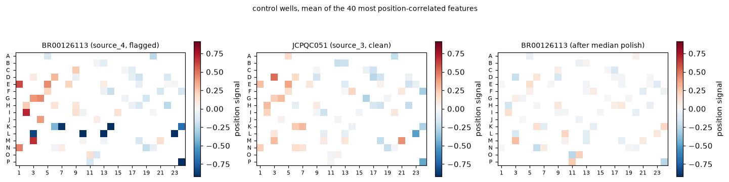
Median polish removes the gradient, as the last panel shows. Whether removing it helps depends on the readout. For compounds we measure cross-source retrieval, which asks whether a compound run at different laboratories is found again. We report it as mean average precision (mAP) against a shuffled null, and we count how many compounds clear the null. The table shows retrieval before and after correcting only the flagged plates.

def cross_source_map(adata):
    """Mean cross-source compound mAP, and how many compounds clear the corrected null."""
    treated = adata[~adata.obs["Metadata_Control"].to_numpy()].copy()
    mt.tl.map(
        treated,
        pos_sameby=["Metadata_Perturbation"],
        pos_diffby=["Metadata_Source"],
        neg_diffby=["Metadata_Perturbation"],
        null_size=500,
        seed=0,
    )
    scores = treated.uns["mantispy"]["map"]
    return round(float(scores["mean_average_precision"].mean()), 3), int(scores["below_corrected_p"].sum())


passing = list(detection.loc[detection["cv_r2_median"] > 0, "plate"])
n_treated = int(jump.obs.loc[~jump.obs["Metadata_Control"].to_numpy(), "Metadata_Perturbation"].nunique())

ladder = {"normalize only": cross_source_map(jump)}
for method in ("median_polish", "b_score"):
    corrected = jump.copy()
    mt.pp.correct_plate_position(corrected, method=method, reference="negcon", plates=passing)
    ladder[f"+ {method} (only the flagged plates)"] = cross_source_map(corrected)

pd.DataFrame(
    [
        {"pipeline": name, "cross-source mAP": value, f"significant of {n_treated}": hits}
        for name, (value, hits) in ladder.items()
    ]
)

	pipeline	cross-source mAP	significant of 301
0	normalize only	0.016	38
1	+ median_polish (only the flagged plates)	0.015	25
2	+ b_score (only the flagged plates)	0.014	21

Correction lowers retrieval. The mAP changes are small, from 0.016 to 0.014 at this seed, but the number of compounds clearing the null falls from 38 to 21. The correction did what it promises and the gradient is gone, yet it is a bad trade on a profile. The row and column fit comes from only a few dozen control wells, so subtracting it adds noise to every treated well. The B-score then rescales each plate by its own MAD on top of the normalization already applied, so a compound is shifted by a different amount on each plate, and cross-source retrieval needs the same amount everywhere. For profiling, normalize per plate, run pp.harmony on the batch, and use detect_plate_position to flag the rare plate worth excluding instead of correcting.

Which method to use

situation	method
hit-calling a single readout against a gradient, randomized layout	correct_plate_position(method="b_score")
removing a gradient while keeping the data’s units	correct_plate_position(method="median_polish")
building multivariate profiles	do not position-correct; normalize per plate and run pp.harmony on the batch
a plate scoring cv_r2_median > 0 on a profiling screen	treat it as a QC flag and exclude or inspect it

For a profiling pipeline:

import scanpy as sc

mt.pp.normalize(adata, method="mad_robustize", by="Metadata_Plate", reference="negcon")
mt.pp.detect_plate_position(adata, reference="negcon")
flagged = adata.uns["mantispy"]["plate_position_detection"].query("cv_r2_median > 0")["plate"]
adata = adata[~adata.obs["Metadata_Plate"].isin(flagged)].copy()
sc.pp.pca(adata, n_comps=50)
mt.pp.harmony(adata, batch_key="Metadata_Batch")

A few caveats sit behind the table.

• Nonrandom layouts. Both methods assume position is independent of treatment. Controls down whole columns, or a dose gradient across columns, is itself the position signal, and correcting it removes the design (Brideau et al. [2003]; median polish fits a column effect only where control wells sit).

• High hit rates. Median polish and the MAD assume most wells are inactive. Many active wells bias the robust centre, and the B-score then compresses real signal.

• The B-score also normalizes. It rescales each plate by its MAD, so run it instead of a separate per-plate normalization, or use median_polish to keep your own.

• Learned correctors are a separate case. For genetic perturbations with deep features, methods like cpDistiller correct well position where the linear correction here does not.

Correct a single readout against a gradient, and do not correct a whole profile. The within-plate mechanics are in the artifacts tutorial.